Understanding Neural Networks: The Brain of AI

Quick Definitions

Before diving in, here are the core terms you’ll encounter throughout this article:

Neuron — The smallest computational unit in a network, inspired by biological brain cells. It receives inputs, processes them, and produces an output.
Weight — A number that controls how much influence a given input has on a neuron’s output. Think of it as the “strength” of a connection.
Activation function — A mathematical gate that decides whether (and how strongly) a neuron “fires.” Common examples include ReLU and sigmoid.
Epoch — One full pass of the entire training dataset through the network, both forward and backward.
Overfitting — When a model memorizes training data so closely that it performs poorly on new, unseen data.

If you’ve ever asked a chatbot to write a paragraph, unlocked your phone with your face, or shopped online and received eerily accurate product recommendations, you’ve interacted with a neural network. Neural networks are computing systems loosely inspired by the architecture of the human brain, and they form the backbone of modern artificial intelligence.

But why do we call them the “brain of AI”? The answer lies in their structure: just as the brain is composed of billions of interconnected neurons that work together to recognize patterns, make decisions, and learn from experience, a neural network is composed of layers of mathematical “neurons” that process information, detect patterns, and improve their performance through training. They’re not a perfect replica of biological brains — far from it — but the analogy holds well enough to give us an intuitive framework.

The difference between neural networks and machine learning as a broader field often confuses newcomers. Machine learning is the umbrella discipline — any system that learns from data qualifies. Neural networks are a specific approach within that umbrella, one that has proven exceptionally powerful for tasks involving images, language, speech, and complex decision-making.

In this article, we’ll walk through how neural networks work from the ground up. You’ll learn about their history, the core mechanics of forward propagation and training, the major neural network architectures used today, and the practical tools you need to start experimenting yourself. Whether you’re a curious professional or an advanced hobbyist, you’ll leave with a solid mental model — and a clear path forward.

Understanding Neural Networks The Brain of AI

History and Background

The story of neural networks stretches back further than most people realize.

From Perceptrons to Deep Learning

In 1949, psychologist Donald Hebb proposed that learning occurs when connections between neurons strengthen through repeated use — an idea formalized as Hebbian learning. A decade later, in 1958, Frank Rosenblatt built the Perceptron, a simple single-layer network capable of classifying inputs into two categories. It generated enormous excitement, with The New York Times proclaiming it “the embryo of an electronic computer that will be able to walk, talk, see, write, reproduce itself and be conscious of its existence.”

That optimism was premature. In 1969, Marvin Minsky and Seymour Papert published a rigorous mathematical critique showing that a single-layer perceptron couldn’t even solve something as simple as an XOR logic gate. Funding dried up, and the field entered its first “AI winter.”

The revival came in the 1980s, when researchers including David Rumelhart, Geoffrey Hinton, and Ronald Williams popularized backpropagation — an algorithm that could efficiently compute how to adjust the weights in a multilayer network to reduce errors. Suddenly, networks with hidden layers could learn complex, nonlinear relationships.

The Deep Learning Explosion

Despite backpropagation, neural networks remained impractical for large-scale problems until the 2010s. Three forces converged:

Massive datasets — The internet generated training data at unprecedented scale (ImageNet alone provided 14 million labeled images).
GPU computing — Graphics processors proved ideal for the parallel matrix operations that neural networks demand.
Algorithmic refinements — Techniques such as dropout, batch normalization, and improved optimizers made deep networks trainable and stable.

The result was a cascade of breakthroughs: AlexNet winning the 2012 ImageNet competition by a wide margin, GPT and BERT revolutionizing natural language processing, and AlphaGo defeating a world champion in Go. Today, deep learning — neural networks with many layers — drives much of the progress in artificial intelligence.

Core Concepts

At their heart, neural networks are relatively simple. They’re made of interconnected layers of nodes (neurons) that pass information forward, adjust their internal parameters, and gradually learn to map inputs to correct outputs. Let’s break down each piece.

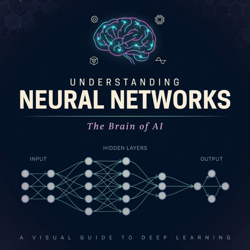
Neurons and Layers

A neuron in an artificial network receives one or more inputs, multiplies each by a weight, adds a bias, and then passes the result through an activation function to produce an output. Conceptually, you can think of neurons as voting members of a committee. Each neuron casts a “vote” on what the input data represents, and the strength of that vote is determined by its weight.

Networks are organized into layers:

Layer	Role
Input layer	Receives raw data (e.g., pixel values, word embeddings)
Hidden layer(s)	Performs intermediate computations; the “thinking” layers
Output layer	Produces the final prediction or classification

The word “deep” in deep learning simply means the network has multiple hidden layers rather than just one.

Weights and Biases

Weights are the heart of learning. A weight is a number that scales an input’s contribution to a neuron. If you imagine the network as a web of roads connecting cities, the weights are the width of each road — wider roads carry more traffic. During training, the network adjusts these weights to minimize errors.

A bias is a constant added to a neuron’s weighted sum before activation. It allows the network to shift the activation threshold — without biases, a neuron could only fire when its inputs collectively reach zero, which would severely limit what the network can learn.

Activation Functions

If a neuron computed only a linear combination of its inputs, the entire network — no matter how many layers — would collapse into a single linear transformation. Activation functions break this limitation by introducing nonlinearity, allowing the network to model complex, curved decision boundaries.

Common activation functions include:

ReLU (Rectified Linear Unit): f(x)=max(0,x). Simple, fast, and the default choice in most modern networks. It lets any positive value pass through and zeros out negatives.
Sigmoid: f(x)=1+e−x1. Squashes any input into the range (0,1), making it useful for binary classification outputs. Rarely used in hidden layers today because it can cause the “vanishing gradient” problem.
Softmax: Converts a vector of numbers into a probability distribution that sums to 1. Standard for the output layer in multi-class classification.

Forward Propagation

Forward propagation is the process of passing input data through the network, layer by layer, to produce an output. For each neuron, the calculation is:

z=i∑wi⋅xi+bthena=f(z)

where wi are weights, xi are inputs, b is the bias, f is the activation function, and a is the output activation.

A Numeric Example: One Forward Pass

Let’s trace a small network step by step. Imagine a network with 2 inputs, 1 hidden layer with 2 neurons (using ReLU), and 1 output neuron (using sigmoid for a probability).

Inputs: x1=0.5,x2=0.8

Hidden layer weights and biases:

	w to h1	w to h2
From x1	0.4	−0.3
From x2	0.6	0.9

Biases: b1=0.1,b2=−0.2

Computing hidden neuron h1:

z1=0.4×0.5+0.6×0.8+0.1=0.20+0.48+0.1=0.78

h1=ReLU(0.78)=0.78

Computing hidden neuron h2:

z2=(−0.3)×0.5+0.9×0.8+(−0.2)=−0.15+0.72−0.2=0.37

h2=ReLU(0.37)=0.37

Output layer (weights w5=0.7,w6=0.5, bias b3=0.05):

zout=0.7×0.78+0.5×0.37+0.05=0.546+0.185+0.05=0.781

Output=sigmoid(0.781)=1+e−0.7811≈0.686

The network’s prediction is approximately 0.686, which we might interpret as a 68.6% probability of belonging to the positive class.

👉 Try it yourself: Change one weight and recompute. You’ll see how sensitive the output is to individual parameters — and why training needs to adjust thousands or millions of them simultaneously.

Loss Functions and Optimization

Once the network produces an output, we need to measure how wrong it is. A loss function does this job:

Mean Squared Error (MSE): Common for regression. Penalizes large errors heavily.
Cross-Entropy Loss: Standard for classification. Measures the divergence between predicted probabilities and true labels.

The goal of training is to minimize the loss by adjusting weights. The primary method is gradient descent, which computes the gradient (slope) of the loss with respect to each weight and nudges the weight in the direction that decreases loss. Variants like Adam and RMSprop add momentum and adaptive learning rates to make convergence faster and more reliable.ct to each weight and nudges the weight in the direction that decreases loss. Variants like Adam and RMSprop add momentum and adaptive learning rates to make convergence faster and more reliable.

Training and Evaluation

The Training Loop

Neural network training follows a cyclical process:

Forward pass: Run input data through the network to get predictions.
Compute loss: Compare predictions to actual labels.
Backpropagation: Propagate the error backward through the network, computing each weight’s contribution to the total error.
Weight update: Adjust weights using gradient descent.
Repeat for many epochs.

Backpropagation is the engine of neural network training. Intuitively, it’s a blame-assignment algorithm: when the network makes a wrong prediction, backprop works backward from the output to figure out which weights were most responsible, then tweaks them proportionally. It relies on the chain rule of calculus to efficiently compute gradients even in deep, multi-layered networks.

Epochs, Batches, and SGD

An epoch is one complete pass through the training set. In practice, we rarely update weights after every single example (stochastic gradient descent) or wait until the entire dataset has been processed (batch gradient descent). Instead, we use mini-batch gradient descent — updating weights after small groups of examples (e.g., 32, 64, or 128 samples). This balances speed and stability.

Overfitting vs. Underfitting

A model that underfits hasn’t learned enough — it’s too simple to capture the patterns in the data. A model that overfits has learned too much — it memorizes noise and specifics of the training set, then fails on new data.

Regularization techniques combat overfitting:

Dropout: Randomly deactivates a percentage of neurons during each training step, forcing the network to learn robust features rather than relying on any single neuron.
L2 regularization (weight decay): Penalizes large weight values, encouraging the network to distribute influence more evenly.

Validation, Testing, and Metrics

Data is typically split into three sets:

Training set — Used to update weights.
Validation set — Used to tune hyperparameters and monitor for overfitting during training.
Test set — Used once, at the end, for a final unbiased performance estimate.

Common metrics include:

Classification: Accuracy, precision, recall, F1-score, AUC-ROC.
Regression: MSE, Mean Absolute Error (MAE), $R^2$.

Types and Architectures

Not all neural networks are built the same way. Different architectures excel at different tasks.

Feedforward Networks (MLPs)

The Multilayer Perceptron (MLP) is the simplest architecture — data flows in one direction from input to output with no cycles. Use cases: tabular data classification, price prediction, basic anomaly detection.

Convolutional Neural Networks (CNNs)

CNNs use convolutional filters that slide across input data (typically images) to detect local patterns like edges, textures, and shapes. Early layers find simple features; deeper layers combine them into complex visual concepts.
Use case: Medical image analysis — detecting tumors in X-rays or MRI scans with accuracy rivaling radiologists.

Recurrent Networks: LSTM and GRU

Recurrent neural networks (RNNs) process sequences by maintaining a hidden state that carries information forward through time. LSTM (Long Short-Term Memory) and GRU (Gated Recurrent Unit) are variants that solve the vanishing gradient problem, allowing the network to learn long-range dependencies.
Use case: Predicting the next word in a sentence, or forecasting stock prices based on historical time series.

Transformers

The transformer architecture, introduced in 2017, replaced recurrence with an attention mechanism — a way for the network to weigh the relevance of every input position to every other position simultaneously. This parallelism makes transformers faster to train and dramatically more capable at handling long-range dependencies.
Use case: Large language models like GPT and BERT that power chatbots, translation, and code generation.

Graph Neural Networks (GNNs)

GNNs operate on graph-structured data, passing messages between nodes connected by edges.
Use case: Drug discovery — predicting molecular properties by treating atoms as nodes and bonds as edges.

Practical Considerations and Tools

Data and Compute

Neural networks are hungry for data and compute. A state-of-the-art image model might need millions of labeled images and weeks of GPU training. For most practitioners, transfer learning is a game-changer: start with a pre-trained model (trained on a massive dataset) and fine-tune it on your smaller, domain-specific data.

Frameworks

Two dominant frameworks power modern deep learning:

PyTorch — Favored by researchers for its dynamic computation graphs and Pythonic feel. Increasingly popular in production as well.
TensorFlow / Keras — Backed by Google, with robust deployment tools (TensorFlow Serving, TFLite, TensorFlow.js).

Both offer high-level APIs that let you build and train models in just a few lines of code.

Deployment and Ethics

Getting a model from a notebook to production involves containerization (Docker), APIs (FastAPI, Flask), and monitoring for data drift. Equally important are ethical considerations:

Bias: Models can inherit and amplify biases present in training data.
Explainability: Research into explainable AI neural networks aims to make model decisions interpretable.
Carbon footprint: Training large models can consume significant energy. Efficiency matters.

Simple Diagram Description

Diagram: Input layer with 3 nodes (blue circles) connected by weighted arrows (thin gray lines) to one hidden layer with 4 nodes (green circles, each labeled “ReLU”). The hidden layer connects via arrows to an output layer with 2 nodes (orange circles, labeled “softmax”). Labels appear beside a few arrows showing sample weight values.

Conclusion and Next Steps

Neural networks have evolved from a mid-century curiosity into the driving force behind modern artificial intelligence. They work by stacking layers of simple, weighted computations — connected by activation functions — and training the whole system through backpropagation and gradient descent. Different architectures serve different needs: CNNs for images, transformers for language, RNNs for sequences, and GNNs for graph data.

If you want to move from understanding to building, here’s a practical roadmap:

Start small: Train an MLP on the MNIST handwritten digits dataset using PyTorch or Keras. It takes under 50 lines of code.
Level up: Try CIFAR-10 (color image classification) with a simple CNN, or the IMDB reviews dataset for sentiment analysis with an LSTM or transformer.
Take a course: Andrew Ng’s Deep Learning Specialization on Coursera and Fast.ai’s Practical Deep Learning are both excellent and freely available.
Experiment: Clone a starter repository on GitHub, swap out the architecture, change hyperparameters, and observe what happens. Intuition comes from breaking things and fixing them.